Exciting new ways to slice and dice your data with Xarray!

import xarray as xr
import numpy as np

xr.set_options(display_expand_indexes=True)

xr.show_versions()

INSTALLED VERSIONS
------------------
commit: None
python: 3.13.5 | packaged by conda-forge | (main, Jun 16 2025, 08:27:50) [GCC 13.3.0]
python-bits: 64
OS: Linux
OS-release: 6.8.0-1029-aws
machine: x86_64
processor: x86_64
byteorder: little
LC_ALL: None
LANG: C.UTF-8
LOCALE: ('C', 'UTF-8')
libhdf5: None
libnetcdf: None

xarray: 2025.6.1
pandas: 2.3.0
numpy: 2.3.1
scipy: 1.16.0
netCDF4: None
pydap: None
h5netcdf: None
h5py: None
zarr: None
cftime: None
nc_time_axis: None
iris: None
bottleneck: None
dask: None
distributed: None
matplotlib: 3.10.3
cartopy: None
seaborn: None
numbagg: None
fsspec: None
cupy: None
pint: None
sparse: None
flox: None
numpy_groupies: None
setuptools: 80.9.0
pip: None
conda: None
pytest: None
mypy: None
IPython: 9.4.0
sphinx: None

What is an index?¶

First thing’s first, what is an index and why is it helpful?

In brief, indexing data makes repeated subsetting and selection more efficient.

Indexing is all around you. In the library you might head straight to section 500 if you’re interested in Natural Sciences and Mathematics. Or 800 if you’re in the mood for a good novel (credit to Dewey, 1876)! Some indexes are less universal and more multi-dimensional: In my local grocery store I know that asile 12, top shelf has the best cereal. And asile 1, second shelf has the yogurt. No need to wander around!

The same efficiencies arise in computing. Consider a simple 1D dataset consisting of measurements Y=[10,20,30,40,50,60] at six positions X=[1, 2, 4, 8, 16, 32]. What was our measurement at X=8?

To extract the answer in code we can loop over all the values of X to find X=8. In Python conventions we find it at position 3, then use that to get our answer Y[3]=40.

PandasIndex¶

So in the above example, the index is simply a key:value mapping between the coordinate values and integer positions i=[0,1,2,3,4,5] in the coordinates array. This in fact is the default Pandas.Index! And this is what Xarray uses behind the scenes to power label-based selection:

# NOTE x in a "PandasIndex"
x = np.array([1, 2, 4, 8, 16, 32])
y = np.array([10, 20, 30, 40, 50, 60])
da = xr.DataArray(y, coords={'x': x})
da

da.sel(x=4).values

Alternatives to PandasIndex¶

Importantly, a loop over all the coordinate values is not the only way to create an index. You might recognize that our coordinates can in fact be represented by a function X(n)=2*n where n is the integer position! Given that information we can evaluate similarly Y(X=4) quickly as Y[2]=30.

RangeIndex¶

Often, coordinates are even simplier and can be definied by a start,stop, and uniform step size. For this, Xarray v2025.03.1 added a built-in RangeIndex that bypasses Pandas. Note that coordinates are now calculated on-the-fly rather than loaded into memory up-front when creating a Dataset.

from xarray.indexes import RangeIndex

index = RangeIndex.arange(0.0, 100_000, 0.1, dim='x')
ds = xr.Dataset(coords=xr.Coordinates.from_xindex(index))
ds

Third-party custom Indexes¶

A lot of work over the last several years has gone into the nuts and bolts of Xarray to make it possible to plug in new Indexes. Here we’ll highlight a few examples!

XProj CRSIndex¶

real-world datasets are usually more than just raw numbers; they have labels which encode information about how the array values map to locations in space, time, etc

Xarray Docs

We often think about metadata providing context for measurement values but metadata is also critical for coordinates! In particular, to align two different datasets we must ask if the coordinates are in the same coordinate system. In other words, do they share the same origin and scale?

There are currently over 7000 commonly used Coordinate Reference Systems (CRS) for geospatial data in the authoritative EPSG database! And of course an infinite number of custom-defined CRSs. xproj.CRSIndex gives Xarray objects an automatic awareness of the coordinate reference system operations like xr.align() no longer succeed when they should raise an error:

from xproj import CRSIndex
lons1 = np.arange(-125, -120, 1)
lons2 = np.arange(-122, -118, 1)
ds1 = xr.Dataset(coords={'longitude': lons1}).proj.assign_crs(crs=4267)
ds2 = xr.Dataset(coords={'longitude': lons2}).proj.assign_crs(crs=4326)
ds1 + ds2

MergeError: conflicting values/indexes on objects to be combined for coordinate 'crs'

Rasterix RasterIndex¶

Earlier we mentioned that coordinates often have a functional representation. For 2D geospatial raster images, this function often takes the form of an Affine Transform. This how the rasterix RasterIndex computes coordinates rather than storing them all in memory. Also alignment by comparing transforms minimizes common errors due to floating point mismatches.

Below is a simple example of slicing a large mosaic of GeoTiffs without ever loading the coordiantes into memory, note that a new Affine is defined after the slicing operation:

# 811816322401 values!
import rasterix

#26475 GeoTiffs represented by a GDAL VRT
da = xr.open_dataarray('https://opentopography.s3.sdsc.edu/raster/COP30/COP30_hh.vrt',
                       engine='rasterio',
                       parse_coordinates=False).squeeze().pipe(
    rasterix.assign_index
)
da

print('Original geotransform:\n', da.xindexes['x'].transform())
da_sliced = da.sel(x=slice(-122.4, -120.0), y=slice(-47.1,-49.0))
print('Sliced geotransform:\n', da_sliced.xindexes['x'].transform())

Original geotransform:
 | 0.00, 0.00,-180.00|
| 0.00,-0.00, 84.00|
| 0.00, 0.00, 1.00|
Sliced geotransform:
 | 0.00, 0.00,-122.40|
| 0.00,-0.00,-47.10|
| 0.00, 0.00, 1.00|

XVec GeometryIndex¶

A “vector data cube” is an n-D array that has at least one dimension indexed by a 2-D array of vector geometries. Large vector cubes can take advantage of an R-tree spatial index for efficiently selecting vector geometries within a given bounding box. The XVec.GeometryIndex provides this functionality, below is a short code snippet but please refer to the documentation for more!

import xvec
import geopandas as gpd
from geodatasets import get_path

# Dataset that contains demographic data indexed by U.S. counties
counties = gpd.read_file(get_path("geoda.natregimes"))

cube = xr.Dataset(
    data_vars=dict(
        population=(["county", "year"], counties[["PO60", "PO70", "PO80", "PO90"]]),
        unemployment=(["county", "year"], counties[["UE60", "UE70", "UE80", "UE90"]]),
    ),
    coords=dict(county=counties.geometry, year=[1960, 1970, 1980, 1990]),
).xvec.set_geom_indexes("county", crs=counties.crs)
cube

# Efficient selection using shapely.STRtree
from shapely.geometry import box

subset = cube.xvec.query(
    "county",
    box(-125.4, 40, -120.0, 50),
    predicate="intersects",
)

subset['population'].xvec.plot(col='year');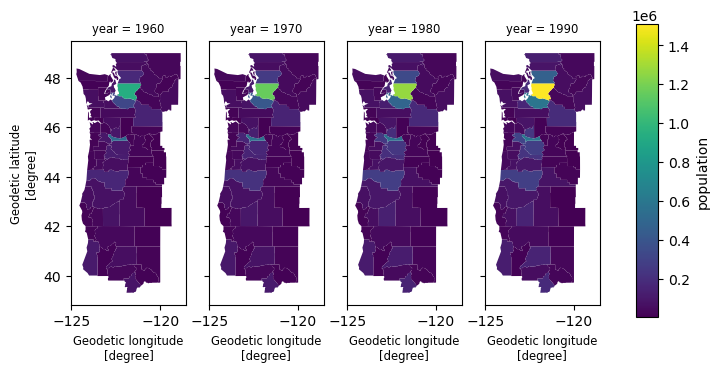

What’s next?¶

While we’re extremely excited about what can already be accomplished with the new indexing capabilities, there are plenty of exciting ideas for future work.

Have an idea for your own custom index? Check out this section of the Xarray documentation, and we recommend following this GitHub Issue.

There are a few new indexes that will soon become part of the Xarray codebase!

• IntervalIndex
• NDPointIndex (KDTree)

We’re working on A Gallery of Custom Index Examples!